Combinations and Permutations

What's the Difference?

In English we use the word "combination" loosely, without thinking if the order of things is important. In other words:

	"My fruit salad is a combination of apples, grapes and bananas" We don't care what order the fruits are in, they could also be "bananas, grapes and apples" or "grapes, apples and bananas", its the same fruit salad.
	"The combination to the safe is 472". Now we do care about the order. "724" won't work, nor will "247". It has to be exactly 4-7-2.

So, in Mathematics we use more precise language:

	When the order doesn't matter, it is a Combination.
	When the order does matter it is a Permutation.

So, we should really call this a "Permutation Lock"!

In other words:

A Permutation is an ordered Combination.

To help you to remember, think "Permutation ... Position"

Permutations

There are basically two types of permutation:

1. Repetition is Allowed: such as the lock above. It could be "333".
2. No Repetition: for example the first three people in a running race. You can't be first and second.

1. Permutations with Repetition

These are the easiest to calculate.

When a thing has n different types ... we have n choices each time!

For example: choosing 3 of those things, the permutations are:

n × n × n (n multiplied 3 times)

More generally: choosing r of something that has n different types, the permutations are:

n × n × ... (r times)

(In other words, there are n possibilities for the first choice, THEN there are n possibilites for the second choice, and so on, multplying each time.)

Which is easier to write down using an exponent of r:

n × n × ... (r times) = n^r

Example: in the lock above, there are 10 numbers to choose from (0,1,2,3,4,5,6,7,8,9) and we choose 3 of them:

10 × 10 × ... (3 times) = 10³ = 1,000 permutations

So, the formula is simply:

nr

where n is the number of things to choose from, and we choose r of them (Repetition allowed, order matters)

2. Permutations without Repetition

In this case, we have to reduce the number of available choices each time.

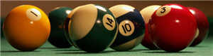
For example, what order could 16 pool balls be in?

After choosing, say, number "14" we can't choose it again.

So, our first choice has 16 possibilites, and our next choice has 15 possibilities, then 14, 13, etc. And the total permutations are:

16 × 15 × 14 × 13 × ... = 20,922,789,888,000

But maybe we don't want to choose them all, just 3 of them, so that is only:

16 × 15 × 14 = 3,360

In other words, there are 3,360 different ways that 3 pool balls could be arranged out of 16 balls.

Without repetition our choices get reduced each time.

But how do we write that mathematically? Answer: we use the "factorial function"

	The factorial function (symbol: !) just means to multiply a series of descending natural numbers. Examples: 4! = 4 × 3 × 2 × 1 = 24 7! = 7 × 6 × 5 × 4 × 3 × 2 × 1 = 5,040 1! = 1
Note: it is generally agreed that 0! = 1. It may seem funny that multiplying no numbers together gets us 1, but it helps simplify a lot of equations.

So, when we want to select all of the billiard balls the permutations are:

16! = 20,922,789,888,000

But when we want to select just 3 we don't want to multiply after 14. How do we do that? There is a neat trick: we divide by 13!

16 × 15 × 14 × 13 × 12 ...		= 16 × 15 × 14 = 3,360
13 × 12 ...

Do you see? 16! / 13! = 16 × 15 × 14

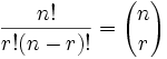
The formula is written:

n!(n − r)!

where n is the number of things to choose from, and we choose r of them (No repetition, order matters)

Example Our "order of 3 out of 16 pool balls example" is:

16!	=	16!	=	20,922,789,888,000	= 3,360
(16-3)!		13!		6,227,020,800

(which is just the same as: 16 × 15 × 14 = 3,360)

Example: How many ways can first and second place be awarded to 10 people?

10!	=	10!	=	3,628,800	= 90
(10-2)!		8!		40,320

(which is just the same as: 10 × 9 = 90)

Notation

Instead of writing the whole formula, people use different notations such as these:

Example: P(10,2) = 90

Combinations

There are also two types of combinations (remember the order does not matter now):

1. Repetition is Allowed: such as coins in your pocket (5,5,5,10,10)
2. No Repetition: such as lottery numbers (2,14,15,27,30,33)

1. Combinations with Repetition

Actually, these are the hardest to explain, so we will come back to this later.

2. Combinations without Repetition

This is how lotteries work. The numbers are drawn one at a time, and if we have the lucky numbers (no matter what order) we win!

The easiest way to explain it is to:

• assume that the order does matter (ie permutations),
• then alter it so the order does not matter.

Going back to our pool ball example, let's say we just want to know which 3 pool balls are chosen, not the order.

We already know that 3 out of 16 gave us 3,360 permutations.

But many of those are the same to us now, because we don't care what order!

For example, let us say balls 1, 2 and 3 are chosen. These are the possibilites:

Order does matter	Order doesn't matter
1 2 3 1 3 2 2 1 3 2 3 1 3 1 2 3 2 1	1 2 3

So, the permutations will have 6 times as many possibilites.

In fact there is an easy way to work out how many ways "1 2 3" could be placed in order, and we have already talked about it. The answer is:

3! = 3 × 2 × 1 = 6

(Another example: 4 things can be placed in 4! = 4 × 3 × 2 × 1 = 24 different ways, try it for yourself!)

So we adjust our permutations formula to reduce it by how many ways the objects could be in order (because we aren't interested in their order any more):

That formula is so important it is often just written in big parentheses like this:

where n is the number of things to choose from, and we choose r of them (No repetition, order doesn't matter)

It is often called "n choose r" (such as "16 choose 3")

And is also known as the Binomial Coefficient.

Notation

As well as the "big parentheses", people also use these notations:

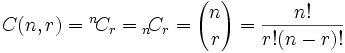
Just remember the formula:

n!r!(n − r)!

Example

So, our pool ball example (now without order) is:

16!	=	16!	=	20,922,789,888,000	= 560
3!(16-3)!		3!×13!		6×6,227,020,800

Or we could do it this way:

16×15×14	=	3360	= 560
3×2×1		6

It is interesting to also note how this formula is nice and symmetrical:

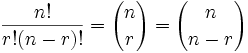
In other words choosing 3 balls out of 16, or choosing 13 balls out of 16 have the same number of combinations.

16!	=	16!	=	16!	= 560
3!(16-3)!		13!(16-13)!		3!×13!

Pascal's Triangle

We can also use Pascal's Triangle to find the values. Go down to row "n" (the top row is 0), and then along "r" places and the value there is our answer. Here is an extract showing row 16:

1    14    91    364  ...

1    15    105   455   1365  ...

1    16   120   560   1820  4368  ...

1. Combinations with Repetition

OK, now we can tackle this one ...

Let us say there are five flavors of icecream: banana, chocolate, lemon, strawberry and vanilla.

We can have three scoops. How many variations will there be?

Let's use letters for the flavors: {b, c, l, s, v}. Example selections include

• {c, c, c} (3 scoops of chocolate)
• {b, l, v} (one each of banana, lemon and vanilla)
• {b, v, v} (one of banana, two of vanilla)

(And just to be clear: There are n=5 things to choose from, and we choose r=3 of them.
Order does not matter, and we can repeat!)

Now, I can't describe directly to you how to calculate this, but I can show you a special technique that lets you work it out.

Think about the ice cream being in boxes, we could say "move past the first box, then take 3 scoops, then move along 3 more boxes to the end" and we will have 3 scoops of chocolate!

So it is like we are ordering a robot to get our ice cream, but it doesn't change anything, we still get what we want.

We can write this down as  (arrow means move, circle means scoop).

In fact the three examples above can be written like this:

{c, c, c} (3 scoops of chocolate):
{b, l, v} (one each of banana, lemon and vanilla):
{b, v, v} (one of banana, two of vanilla):

OK, so instead of worrying about different flavors, we have a simpler question: "how many different ways can we arrange arrows and circles?"

Notice that there are always 3 circles (3 scoops of ice cream) and 4 arrows (we need to move 4 times to go from the 1st to 5th container).

So (being general here) there are r + (n−1) positions, and we want to choose r of them to have circles.

This is like saying "we have r + (n−1) pool balls and want to choose r of them". In other words it is now like the pool balls question, but with slightly changed numbers. And we can write it like this:

where n is the number of things to choose from, and we choose r of them (Repetition allowed, order doesn't matter)

Interestingly, we can look at the arrows instead of the circles, and say "we have r + (n−1) positions and want to choose (n−1) of them to have arrows", and the answer is the same:

So, what about our example, what is the answer?

(3+5−1)!	=	7!	=	5040	= 35
3!(5−1)!		3!×4!		6×24

In Conclusion

Phew, that was a lot to absorb, so maybe you could read it again to be sure!

But knowing how these formulas work is only half the battle. Figuring out how to interpret a real world situation can be quite hard.

But at least now you know how to calculate all 4 variations of "Order does/does not matter" and "Repeats are/are not allowed".

QUESTION

Q.1

Jones is the Chairman of a committee. In how many ways can a committee of 5 be chosen from 10 people given that Jones must be one of them?

A

126

B

252

C

495

D

3,024

Q.2

How many permutations of 4 different letters are there, chosen from the twenty six letters of the alphabet?

A

14,950

B

23,751

C

358,800

D

456,976

Q.3

How many permutations of 3 different digits are there, chosen from the ten digits 0 to 9 inclusive?

(Such as drawing ten numbered marbles from a bag, without replacement)

A

84

B

120

C

504

D

720

Probability

How likely something is to happen.

Many events can't be predicted with total certainty. The best we can say is how likely they are to happen, using the idea of probability.

Tossing a Coin  When a coin is tossed, there are two possible outcomes: heads (H) or tails (T) We say that the probability of the coin landing H is ½. And the probability of the coin landing T is ½.

Throwing Dice  When a single die is thrown, there are six possible outcomes: 1, 2, 3, 4, 5, 6. The probability of any one of them is 1/6.

Probability 

In general:

Probability of an event happening = Number of ways it can happenTotal number of outcomes

Example: the chances of rolling a "4" with a die

Number of ways it can happen: 1 (there is only 1 face with a "4" on it)

Total number of outcomes: 6 (there are 6 faces altogether)

So the probability = 16

Example: there are 5 marbles in a bag: 4 are blue, and 1 is red. What is the probability that a blue marble gets picked?

Number of ways it can happen: 4 (there are 4 blues)

Total number of outcomes: 5 (there are 5 marbles in total)

So the probability = 45 = 0.8

Probability Line

We can show probability on a Probability Line:

Probability is always between 0 and 1

Probability is Just a Guide

Probability does not tell us exactly what will happen, it is just a guide

Example: toss a coin 100 times, how many Heads will come up?

Probability says that heads have a ½ chance, so we can expect 50 Heads.

But when we actually try it we might get 48 heads, or 55 heads ... or anything really, but in most cases it will be a number near 50.

Learn more at Probability Index.

Words

Some words have special meaning in Probability:

Experiment or Trial: an action where the result is uncertain.

Tossing a coin, throwing dice, seeing what pizza people choose are all examples of experiments.

Sample Space: all the possible outcomes of an experiment

Example: choosing a card from a deck

There are 52 cards in a deck (not including Jokers)

So the Sample Space is all 52 possible cards: {Ace of Hearts, 2 of Hearts, etc... }

The Sample Space is made up of Sample Points:

Sample Point: just one of the possible outcomes

Example: Deck of Cards

• the 5 of Clubs is a sample point
• the King of Hearts is a sample point

"King" is not a sample point. As there are 4 Kings that is 4 different sample points.

Event: a single result of an experiment

Example Events:

• Getting a Tail when tossing a coin is an event
• Rolling a "5" is an event.

An event can include one or more possible outcomes:

• Choosing a "King" from a deck of cards (any of the 4 Kings) is an event
• Rolling an "even number" (2, 4 or 6) is also an event

The Sample Space is all possible outcomes. A Sample Point is just one possible outcome. And an Event can be one or more of the possible outcomes.

Hey, let's use those words, so you get used to them:

Example: Alex wants to see how many times a "double" comes up when throwing 2 dice.

Each time Alex throws the 2 dice is an Experiment.

It is an Experiment because the result is uncertain.

The Event Alex is looking for is a "double", where both dice have the same number. It is made up of these 6 Sample Points:

{1,1} {2,2} {3,3} {4,4} {5,5} and {6,6}

The Sample Space is all possible outcomes (36 Sample Points):

{1,1} {1,2} {1,3} {1,4} ... {6,3} {6,4} {6,5} {6,6}

These are Alex's Results:

Experiment	Is it a Double?
{3,4}	No
{5,1}	No
{2,2}	Yes
{6,3}	No
...	...

After 100 Experiments, Alex has 19 "double" Events ... is that close to what you would expect?


QUESTION

Q.1

A card is chosen at random from a deck of 52 playing cards. 

There are 4 Queens and 4 Kings in a deck of playing cards.

What is the probability the card chosen is a Queen or a King?

Q.2


The diagram shows a spinner made up of a piece of card in the shape of a regular pentagon, with a toothpick pushed through its center. The five triangles are numbered from 1 to 5.

The spinner is spun until it lands on one of the five edges of the pentagon. What is the probability that the number it lands on is odd?

Q.3

A die is thrown once. What is the probability that the score is a factor of 6?

A

1/6

B

1/2

C

2/3

D

1

Measure of dispersion

Measures of Dispersion

It is possible to have two very different datasets with the same means and medians. For that reason, measures of the middle are useful but limited. Another important attribute of a dataset is its dispersion or variability about its middle. The most useful measures of dispersion are the range, percentiles, and the standard deviation. The range is the difference between the largest and the smallest data values. Therefore, the more spread out the data values are, the larger the range will be. However, if a few observations are relatively far from the middle but the rest are relatively close to the middle, the range can give a distorted measure of dispersion.
Percentiles are positional measures for a dataset that enable one to determine the relative standing of a single measurement within the dataset. In particular, the  is defined to be a number such that  of the observations are less than or equal to that number and  are greater than that number. So, for example, an observation that is at the  is less than only 25% of the data. In practice, we often cannot satisfy the definition exactly. However, the steps outlined below at least satisfies the spirit of the definition.

1. Order the data values from smallest to largest; include ties.
2. Determine the position, 
   
   
   
   
3. The  is located between the  and the  ordered value. Use the fractional part of the position, .ddd as an interpolation factor between these values. If k = 0, then take the smallest observation as the percentile and if , then take the largest observation as the percentile. For example, if n = 75 and we wish to find the  percentile, then the position is. The percentile is then located between the  and  ordered values. Suppose that these are 57.8 and 61.3, respectively. Then the percentile would be 
   
   
   
   

Note. Quantiles are equivalent to percentiles with the percentile expressed as a proportion (  is the  quantile).
The  percentile is the median and partitions the data into a lower half (below median) and upper half (above median). The , ,  percentiles are referred to as quartiles. They partition the data into 4 groups with 25% of the values below the  percentile (lower quartile), 25% between the lower quartile and the median, 25% between the median and the  percentile (upper quartile), and 25% above the upper quartile. The difference between the upper and lower quartiles is referred to as the inter-quartile range. This is the range of the middle 50% of the data.
The third measure of dispersion we will consider here is associated with the concept of distance between a number and a set of data. Suppose we are interested in a particular dataset and would like to summarize the information in that data with a single value that represents the closest number to the data. To accomplish this requires that we first define a measure of distance between a number and a dataset. One such measure can be defined as the total distance between the number and the values in the dataset. That is, the distance between a number c and a set of data values, , would be 

It can be shown that the value that minimizes D(c) is the median. However, this measure of distance is not widely used for several reasons, one of which is that this minimization problem does not always have a unique solution.
An alternative measure of distance between a number and a set of data that is widely used and does have a unique solution is defined by, 

That is, the distance between a number c and the data is the sum of the squared distances between c and each data value. We can take as our single number summary the value of c that is closest to the dataset, i.e., the value of c which minimizes . It can be shown that the value that minimizes this distance is . This is accomplished by differentiating D(c) with respect to c and setting the derivative equal to 0. 

As we have already seen, the solution to this equation is . The graphic below gives a histogram of the Weight data with the distance function D(c) superimposed. This graph shows that the minimum distance occurs at the mean of Weight.
 
The mean is the closest single number to the data when we define distance by the square of the deviation between the number and a data value. The average distance between the data and the mean is referred to as the variance of the data. We make a notational distinction and a minor arithmetic distinction between variance defined for populations and variance defined for samples. We use 

for population variances, and 

for sample variances. Note that the unit of measure for the variance is the square of the unit of measure for the data. For that reason (and others), the square root of the variance, called the standard deviation, is more commonly used as a measure of dispersion, 

Note that datasets in which the values tend to be far away from the middle have a large variance (and hence large standard deviation), and datasets in which the values cluster closely around the middle have small variance. Unfortunately, it is also the case that a data set with one value very far from the middle and the rest very close to the middle also will have a large variance.
The standard deviation of a dataset can be interpreted by Chebychev's Theorem:

for any , the proportion of observations within the interval  is at least .

For example, the mean of the Mileage data is 24.583 and the standard deviation is 4.79. Therefore, at least 75% of the cars in this dataset have weights between  and . Chebychev's theorem is very conservative since it is applicable to every dataset. The actual number of cars whose Mileage falls in the interval (15.003,34.163) is 58, corresponding to 96.7%. Nevertheless, knowing just the mean and standard deviation of a dataset allows us to obtain a rough picture of the distribution of the data values. Note that the smaller the standard deviation, the smaller is the interval that is guaranteed to contain at least 75% of the observations. Conversely, the larger the standard deviation, the more likely it is that an observation will not be close to the mean. From the point of view of a manufacturer, reduction in variability of some product characteristic would correspond to an increase of consistency of the product. From the point of view of a financial manager, variability of a portfolio's return is referred to as volatility.
Note that Chebychev's Theorem applies to all data and therefore must be conservative. In many situations the actual percentages contained within these intervals are much higher than the minimums specified by this theorem. If the shape of the data histogram is known, then better results can be given. In particular, if it is known that the data histogram is approximately bell-shaped, then we can say
 contains approximately 68%,
 contains approximately 95%,
 contains essentially all
of the data values. This set of results is called the empirical rule. Later in the course we will study the bell-shaped curve (known as the normal distribution) in more detail.
The relative position of an observation in a data set can be represented by its distance from the mean expressed in terms of the s.d. That is, 

and is referred to as the z-score of the observation. NPositive z-scores are above the mean, negative z-scores are below the mean. Z-scores greater than 2 are more than 2 s.d.'s above the mean. From Chebychev's theorem, at least 75% of observations in any dataset will have z-scores between -2 and 2
Since z-scores are dimension-less, then we can compare the relative positions of observations from different populations or samples by comparing their respective z-scores. For example, directly comparing the heights of a husband and wife would not be appropriate since males tend to be taller than females. However, if we knew the means and s.d.'s of males and females, then we could compare their z-scores. This comparison would be more meaningful than a direct comparison of their heights.
If the data histogram is approximately bell-shaped, then essentially all values should be within 3 s.d.'s of the mean, which is an interval of width 6 s.d.'s. A small number of observations that are unusually large or small can greatly inflate the s.d. Such observations are referred to as outliers. Identification of outliers is important, but this can be difficult since they will distort the mean and the s.d. For that reason, we can't simply use  or  for this purpose. We instead make use of some relationships between quartiles and the s.d. of bell-shaped data. In particular, if the data histogram is approximately bell-shaped, then . This relationship can be used to define a robust estimate of the s.d. which is then used to identify outliers. Observations that are more than  from the nearest quartile are considered to be outliers. Boxplots in R are constructed so that the box edges are at the quartiles, the median is marked by a line within the box, and this the box is extended by whiskers indicating the range of observations that are no more than 1.5(IQR) from the nearest quartile. Any observations falling outside this range are plotted with a circle. For example, the following plot shows boxplots of mileage for each automobile type.